This is the homepage of Peter Alexander. I am currently at Facebook working on AR/VR. Any opinions are my own.

Recent Posts

• Single-Threaded Parallelism
• unique_ptr Type Erasure
• The Condenser Part 1
• Cube Vertex Numbering
• Range-Based Graph Search in D

Links

Single-Threaded Parallelism

Modern computers are able to go fast by doing many things at the same time. We often ask computers to do things at the same time by running code on different threads, but even on a single thread a computer is able to do a lot of things in parallel. One way it does this is by continuing to execute instructions while waiting for a memory access from a previous instruction to complete. This is called out of order execution.

Computers can only execute an instruction while waiting for a memory access if the instruction itself does not depend on the result of the memory access. For example, in C, loading a value through pointers such as a->b->c, we must first wait for the pointer a->b to be loaded before loading ->c. These cannot be loaded out of order, and this slows us down. Serialising memory accesses this way is called pointer chasing. It is a common source of performance issues.

How slow can it be? I wrote a benchmark that simulates pointer chasing by jumping around an array. The main loop is:

int k = 100_000_000;
size_t i = 0;
while (k--) {
  i = a[i];
}

The array a contains the integers 0 .. n, which are shuffled using Sattolo’s algorithm to contain a single cycle permutation. This ensures that every index of a is hit and that there’s no way for the computer to try and predict what memory to fetch next.

The benchmark will depend on the size of the array. Smaller arrays will fit in cache, where memory access latency is significantly smaller. I have run the benchmark for many different array sizes.

Note that in all runs we are doing 100M iterations of that array. The only difference between runs is the size of the array. The time to perform 100M iterations between the smallest array and largest is nearly 100x (both axes are logarithmic). Cache hit rates have a very significant affect on performance.

Is this task memory bound? At the right of the chart, the benchmark is running for around 14 seconds, each iteration is loading 64 bytes of memory (memory operates on cache lines rather than bytes). Putting this together, we are loading 6.4GB in 14 seconds, which is just over 450MB/s. Memory bandwidth is usually on the order of tens of gigabytes per second, so we are far from being memory bound.

The benchmark is slow because the memory accesses are serialised through pointer chasing. To go faster, we need to parallelise. We cannot parallelise this task without changing the underlying data structure, but we could run multiple of these tasks in parallel. We could use threads for this, but can we parallelise on a single thread? What if we iterated with two indices at the same time?

The next benchmark creates two permuted arrays (a and b) with the same combined size as the single array a from the previous benchmark. The iteration is then changed to:

int k = 100_000_000;
size_t i = 0;
size_t j = 0;
while (k--) {
  i = a[i];
  j = b[j];
}

Note that we are still doing the same number of iterations, but with twice as many total lookups. How does this compare?

The times are very similar. On average, the second benchmark is less than 10% slower than the first benchmark, but is doing twice as much work! This scales because the memory loads from a and b can be done in parallel, even from a single thread.

We continue to see good scaling even with eight lookups per iteration.

Amdahl’s Law is starting to kick in at smaller data sizes, but at larger sizes we still see significant gains from parallelism.

Memory access can have high latency, especially as the working set size of our programs increases. Computers try to compensate for memory latency by executing other instructions in parallel while waiting for memory accesses to complete, but they can only do this is there is other work that can be done without waiting. There are significant performance gains to be had by ensuring work is always available to be done, and the programmer plays a role in organising code so that this happens.

unique_ptr Type Erasure

Often when building APIs we’d like the caller to provide some information in a format, or using a protocol defined by the library. For example, we might want access to a contiguous buffer specified by a (void*, size_t) pair.

void cool_feature(void* buffer, size_t len);

An API like this is fine if the buffer will be read synchonously, but sometimes we need asynchronous access. This introduces a lifetime problem: how does the caller know when it can free the buffer?

A common way to solve this is to provide a callback that will be invoked once the processing has completed:

void cool_feature(void* buffer, size_t len, void (*done)(void*));

Here, done will be called with buffer once cool_feature has asynchonously finished its work.

This works most of the time, but has a couple of problems:

1. You need to remember to call done in all cases.
2. It only works if done only needs to be called with the buffer pointer. What if my buffer is part of a larger object?

struct Object {
  // ...
  std::string buffer;
  // ...
};

void do_stuff(std::unique_ptr<Object> obj) {
  cool_feature(obj.buffer.data(), obj.buffer.size(), ???);
}

There’s no obvious choice of function to pass in. We want to free obj once buffer processing is done, but we’ll be given a pointer to the string data, not obj.

A possible solution is to pass in an std::function<void()> as the callback, so that obj can be captured and destroyed as necessary. This works, but std::function has difficulty with move-only types, and there’s no guarantees that a capturing std::function won’t allocate memory.

We could, of course, define another interface (maybe call it ContiguousBufferProvider), but this also requires an extra memory allocation.

A little trick we can do to handle most of the common cases is to pass in a type-erased context to the function.

using Context = std::unique_ptr<void*, void(*)(void*)>;

void cool_feature(void* buffer, size_t len, Context context);

The context is essentially an extra piece of baggage that must be carried around until the buffer has been processed. Once processed, we just drop the context and it cleans up after itself.

We can also benefit from an extra function that converts any object into a Context through type erasure:

template <typename T>
void deleter(void* p) {
  delete static_cast<T*>(p);
}

template <typename T>
Context erase_type(std::unique_ptr<T> p) {
  return Context(static_cast<void*>(p.release()), &deleter<T>);
}

With this, the Object example is easy to solve:

void do_stuff(std::unique_ptr<Object> obj) {
  cool_feature(
      obj.buffer.data(),
      obj.buffer.size(),
      erase_type(std::move(obj));
}

This guarantees no extra memory allocations, and cool_feature just needs to drop the context once finished.

There are probably more general ways to solve this, but I like this approach as it is clean, simple, and solves all the problems I’ve encountered so far.

The Condenser Part 1

Last night I rewatched Joe Armstrong’s excellent keynote from this year’s Strange Loop conference. He begins the talk with a fairly standard, but humorous lament about the sorry state of software, then goes on to relate this to some physical quantities and limits. He finishes by suggesting some possible directions we can look to improve things.

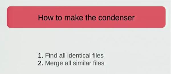
One of his suggestions is to build something called “The Condenser”, which is a program that takes all programs in the world, and condenses them down in such a way that all redundancy is removed. He breaks this task down into two parts:

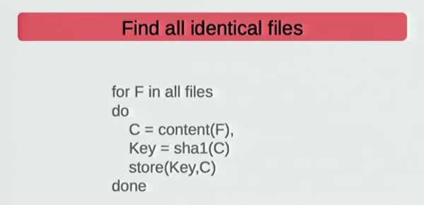
He also explains the obvious, and easy way to do Part 1.

At this point I remembered that I hadn’t written a lot of D recently, and although Joe is talking about condensing all files in the world, I was kind of curious how much duplication there was just on my laptop. How many precious bytes am I wasting?

It turns out that The Condenser Part 1 is very easy to write in D, and even quite elegant.

import std.algorithm;
import std.digest.sha;
import std.file;
import std.parallelism;
import std.stdio;
import std.typecons;

auto process(DirEntry e) {
  ubyte[4 << 10] buf = void;  // 4kb buffer, uninitialized
  auto sha1 = File(e.name).byChunk(buf[]).digest!SHA1;
  return tuple(e.name, sha1, e.size);
}

void main(string[] args) {
  string[ubyte[20]] hash2file;  // hash table of SHA1 -> filename
  auto files = dirEntries(args[1], SpanMode.depth, false)
               .filter!(e => e.isFile);
  foreach (t; taskPool.map!(process)(files)) {
    if (string* original = t[1] in hash2file) {
      writefln("%s %s duplicates %s", t[2], t[0], *original);
    } else {
      hash2file[t[1]] = t[0];
    }
  }
}

I’ll explain the code a little, starting from main. The files variable uses dirEntries and filter to produce a list of files (the filter is necessary since dirEntries also returns directories). dirEntries is a lazy range, so the directories are only iterated as necessary. Similarly, filter creates another lazy range, which removes non-file entries.

The foreach loop corresponds to Joe’s do loop. While I could have just iterated over files directly, I instead iterate over a taskPool.map, a semi-lazy map from David Simcha’s std.parallelism that does the processing in parallel on multiple threads. It is semi-lazy because it eagerly takes a chunk of elements at a time from the front of the range, processes them in parallel, then returns them back to the caller to consume. The task pool size defaults to the number of CPU cores on your machine, but this can be configured.

The process function is where the hashing is done. It takes a DirEntry, allocates an uninitialized (= void) 4kb buffer on the stack and uses that buffer to read the file 4kb at a time and build up the SHA1. Again, byChunk returns a lazy range, and digest!SHA1 consumes it. Lazy ranges are very common in idiomatic D, especially in these kinds of stream processing type applications. It’s worth getting familiar with the common ranges in std.algorithm and std.range.

I ran the program over my laptop’s home directory. Since the duplicate file sizes are all in the first column, I can just use awk to sum them up and find the total waste:

$ sudo ./the-condenser . | awk '{s+=$1} END {print s}'
2347353793

That’s 2.18Gb of duplicate files, which is around 10% of my home dir.

In some cases the duplicates are just files that I have absentmindedly downloaded twice. In other cases it’s duplicate music that I have both in iTunes and Google Play. For some reason, the game Left 4 Dead 2 seems to have a lot of duplicate audio files.

So, in theory, I could save 10% by deduplicating all these files, but it’s not a massive amount of waste. It doesn’t seem worth the effort trying to fix this. Perhaps it would be nice for the OS or file system to solve this automatically, but the implementation would be tricky, and still maybe not worth it.

Part 2 of the Condenser is to merge all similar files using least compression difference. This is decidedly more difficult, since it relies on near-perfect compression, which is apparently an AI-hard problem. Unfortunately, solving AI is out of scope for this post, so I’ll leave that for another time :-)

Cube Vertex Numbering

If you do any sort of graphics, physics, or 3D programming in general then at some point you are going to be working with cubes, and at some point you are going to need to assign a number to each vertex in those cubes. Usually this is because you need to store them in an array, or maybe you are labelling the children of an octree, but often you just need some consistent way of identifying vertices.

For whatever reason, a surprisingly common way of numbering vertices is like this, with the bottom vertices numbered in counter-clockwise order followed by the top vertices in counter-clockwise order (warning, incoming ASCII art):

        7-------6
       /|      /|
      4-+-----5 | 
      | |     | |   y
      | 3-----+-2   | z
      |/      |/    |/
      0-------1     +--x

Depending on what you are doing, there’s generally only a few applications of the numbering system:

• Converting a number to a coordinate.
• Converting a coordinate to a number.
• Enumerating adjacent vertex numbers.

Unfortunately, this common numbering scheme makes none of these tasks easy, and you have no choice but to produce tables of coordinates and adjacency lists for each vertex number. This is tedious, error-prone, and completely unnecessary.

Here is a better scheme:

        3-------7
       /|      /|
      2-+-----6 | 
      | |     | |   y
      | 1-----+-5   | z
      |/      |/    |/
      0-------4     +--x

This numbering uses the Lexicographic Ordering of the vertices, with 0 being the lexicographically first vertex, and 7 being the last.

I’ve included the binary representation of the vertex number in table above, because it illuminates the key property of this scheme: the coordinate of a vertex is equal to the binary representation its vertex number.

\[ \begin{aligned} coordinate(n) &= ((n \gg 2) \mathrel{\&} 1, (n \gg 1) \mathrel{\&} 1, (n \gg 0) \mathrel{\&} 1) \\ number(x, y, z) &= (x \ll 2) \mathrel{|} (y \ll 1) \mathrel{|} (z \ll 0) \end{aligned} \]

(Of course, the zero shifts are unnecessary, but I’ve added them to highlight the symmetry.)

This numbering scheme also makes adjacent vertex enumeration easy. As an adjacent vertex is just a vertex that differs along one axis, we just need to flip each bit using XOR to get the adjacent vertices:

\[ \begin{aligned} adj_x(n) &= n \oplus 100_2 \\ adj_y(n) &= n \oplus 010_2 \\ adj_z(n) &= n \oplus 001_2 \end{aligned} \]

It should be clear that this numbering scheme trivially extends into higher dimension hypercubes by simply using more bits in the representation, and extending the formulae in obvious ways.

So there you have it. Whenever you are looking to number things and aren’t sure what order to use, start with lexicographic. It usually has nice encoding and enumeration properties, and if not then it is probably no worse than any other ordering.

Range-Based Graph Search in D

I’ve just made my first commit of a range-based graph library for D. At the moment it only contains a few basic search algorithms (DFS, BFS, Dijsktra, and A*), but I wanted to write a bit about the design of the library, and how you can use it.

As a bit of a teaser, the snippet below shows how you can use the library to solve those word change puzzles (you know, the ones when you have to get from one word to another by only changing one letter at a time?)

string[] words = File("/usr/share/dict/words")
                 .byLine
                 .filter!(w => w.length == 5)
                 .map!"a.idup"
                 .array();
enum string start = "hello";
enum string end = "world";
static d(string a, string b) { return zip(a, b).count!"a[0] != a[1]"; }
auto graph = implicitGraph!(string, u => words.filter!(v => d(u, v) == 1));
graph.aStarSearch!(v => d(v, end))(start).find(end).path.writeln();

This promptly produces the desired result:

["hello", "hollo", "holly", "molly", "mouly", "mould", "would", "world"]

The last two lines are the interesting part. The first of those lines defines our graph as an implicit graph of words connected by one-letter changes. The second line performs the A* search and writes the resultant path to stdout.

On the second-last line, graph is defined as an implicitGraph. An implicit graph is a graph that is represented by functions rather than in-memory data structures. Instead of having an array of adjacency lists, we just define a function that returns a range of adjacent words (that’s the second parameter to implicitGraph). This representation saves us the tedium of generating the graph beforehand, and saves your RAM from having to store it unnecessarily. It also makes for succinct graph definitions!

The last line is where the algorithm is called. Unlike most other graph libraries, stdex.graph implements graph searches as ranges – iterations of the graph vertices. aStarSearch returns a range of vertices in the order they would be visited by the A* search algorithm (parameterized by the A* heuristic). By implementing the search as a range, the user can take advantage of Phobos’ multitude of range algorithms.

For instance, suppose you want to count the number of nodes searched by the algorithm until it reaches the target node. For this task, you can just use countUntil from std.algorithm.

auto search = graph.aStarSearch!(v => d(v, end))(start);
writefln("%d nodes visited", search.countUntil(end));

For tuning and debugging, it might be useful to print out the nodes visited by the algorithm as it runs.

foreach (node; search.until(end))
    writeln(node);

When no path is available, graph search algorithms typically end up searching the entire vertex space. It is common to cut-off the search after a certain threshold of nodes have been searched. This can be accomplished by takeing only so many nodes from the search.

auto result = search.take(50).find(end);
if (result.empty)
    writeln("Not found within 50 nodes");

Similarly, you could have the search continue until 10 seconds have elapsed.

alias now = TickDuration.currSystemTick;
auto t = now;
auto result = search.until!(_ => (now - t).seconds > 10).find(end);
if (result.empty)
    writeln("Not found in 10 seconds");

The beauty of all this is that none of these features are part of the graph library – they come for free as a side-effect of being a range.

One unsolved part of the design for the graph searches is how to handle visitation. The Boost Graph Library solves this by having users implement a visitor object, which has to define a suite of callback methods, one for each event (vertex discovered, examine edge, etc.) This is certainly mimicable in D, but it may be more effective to model visitation with output ranges, which would again allow composition with existing Phobos constructs. This is what I will be investigating next.